Real-time Aggregate Flexibility

Motivation

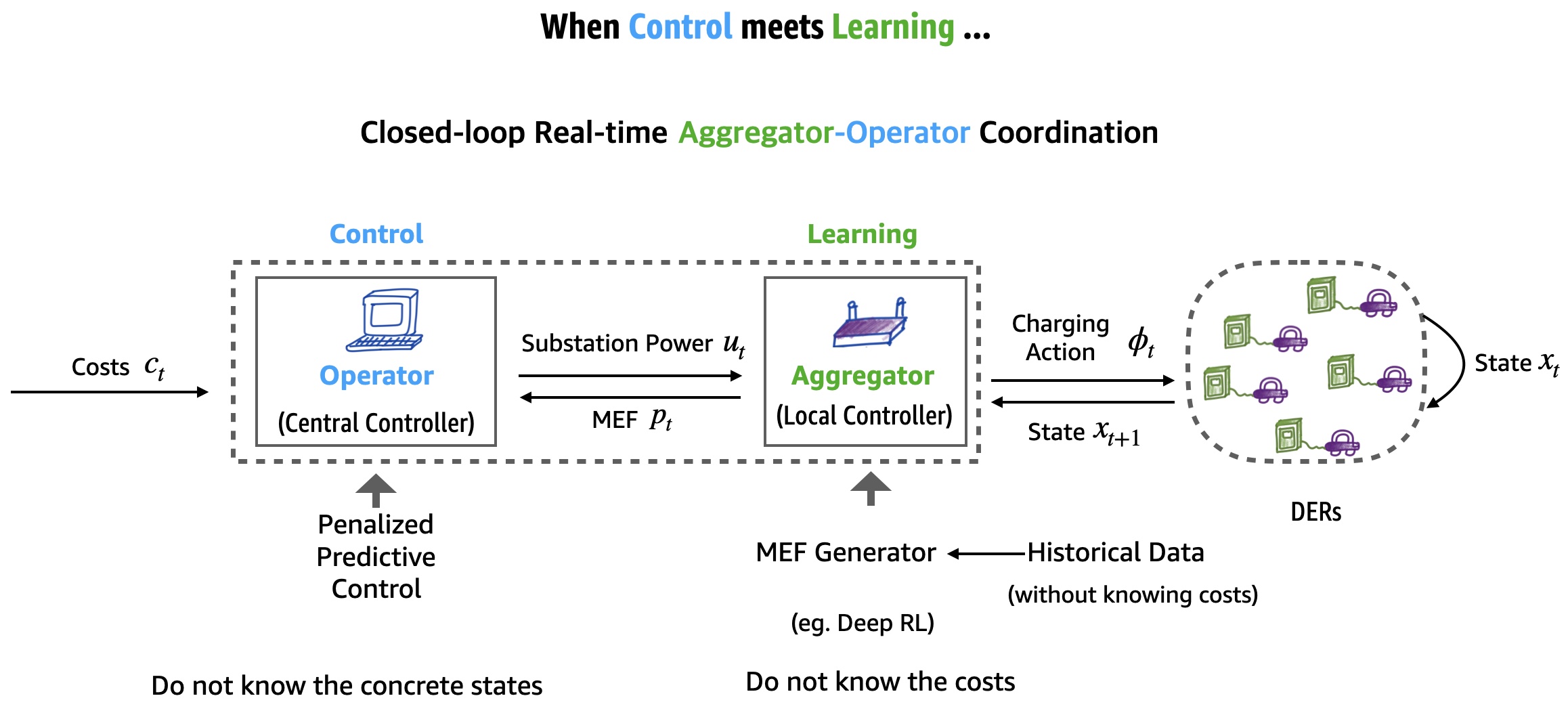
In a real-world control system, there might be hundreds or thousands of controllable units. The units, such as electric vehicle supply equipments (EVSEs) in an EV charging network cannot be controlled in a distributed way because their integrated chips are typically not powerful enough to perform the computations. To minimize both the communication and computational complexity and reduce the leakage of private information, it is of practical importance to introduce a intermediate aggregator that provides information aggregation service to a system operator (such as the California ISO) to make its life easier.

A Control + Learning Framework

It is therefore vital to have a real-time implementation of such a aggregator-operator coordination. We consider a novel definition of real-time aggregate flexibility by an entropic maximization-based approach (which will be expained throughoutly in the next section). In our design, the controller (called an operator in our model) and aggregator together form a closed-loop control system and the feedback is learned from data based on its mathematical definition. The system is presented below and more details can be found in the reference [1] listed at the bottom of the page.

A Novel Information-theoretic Measure of Flexibility

The framework above relies on a real-time measure of flexibility of DERs, i.e., the notion \(p_t\) in the figure above. In the sequel, we introduce a new idea of defining this flexibility measure.

The traditional approaches

Traditional flexibility evaluation methods mostly consider measures that are offline convex approximations of feasible sets of actions (such as substation power \(u_t\) in the above figure). For example, consider a set \(\mathsf{S}\) of feasible actions \((u_1,\ldots,u_T)\) where each \(u_t\in\mathsf{U}\) is some feasible action at time \(t\) chosen from a set of actions \(\mathsf{U}\) that can be either discrete or continuous. Note that the size of \(\mathsf{S}\) measures the level of flexibility, a.k.a the power of selecting different action trajectories. An idea for flexibility evaluation is to measure the lower and upper bounds on the actions such that an interval

for some \(v_{t+1}, \ldots, v_{T}\) where \(u_{< t}:=(u_1,\ldots,u_{t-1})\) is a subsequence denoting selected actions at previous times \(1,\ldots,t-1\). Roughly speaking, \(\mathcal{I}_{t}(u_{< t})\) defines an interval where the current action \(u_t\) can be chosen from. This way of defining flexibility via upper and lower bounds has been widely studied and applied in literature for solving optimizations [2] and flexibility market design [3], etc. Mathematically, the upper and lower bounds \(\mathcal{I}_{t}\) at all times \(t=1,\ldots, T\), together form a hyper-rectangular approximation. Note that some more accurate flexibility representations as better convex approximations do exist, such as [3]. But as a convex approximation, it is not clear how to represent flexibility in real-time, that is, how to measure the system’s flexibility at each time \(t\) using the defined notions.

Generalizing lower and upper bound representations …

Let us consider a more general setting where \(\mathsf{S}\) can be any measurable set. In this case, at each time, the feasible set consisting of \(u_t\) may not be an interval. Therefore, finding a better yet simple flexibility measure is an interesting problem.

An intuitive idea is to generalize the notion of “intervals” defined at each time step using a probability distribution, which may be non-uniform. To illustrate this idea, let us consider a simple example. Let \(\mathcal{U}_t\in\mathbb{R}\) be a set of possible choices of actions at time \(t\). The upper of lower bound flexibility representation would find some \(a\) and \(b\) such that \(a\leq u\) and \(u\leq b\) for any \(u\in\mathcal{U}_t\). Therefore, to generalize it, What if we define a non-uniform distribution on \(\text{ }\mathcal{U}_t?\) In practice, the action space \(\mathsf{U}\) is often a bounded domain such as a set of a few substation power levels or setpoints. This is equivalent to, say, defining a weight for each of the possible choices of substation levels. In this way, the previous widely used notions of bounds can be regarded as assigning equal weights to feasible choices (where the infeasible choices are assigned with a weight \(0\)).

Hence, let \(p_t(u_{<t})\) denote such a generalization of feasible intervals using weights. In fact, when the action space \(\mathsf{U}\) is discrete, \(p_t(u_{<t})\) is a conditional distribution that depends on previous actions that haven been taken \(u_{<t}\); when \(\mathsf{U}\) is continuous, \(p_t(u_{<t})\) is a conditional density function. In many real-world applications, \(\mathsf{U}\) is bounded and can often be discretized. Therefore, in our following discussions, we assume without loss of generality \(\mathsf{U}\) is discrete and \(p_t(u_{<t})\) is thus a probability vector when \(u_{<t}\) is fixed. The action \(u_t\) is a random variable whose event space is the action space \(\mathsf{U}\).

The remaining question is how to define the weights of the probability vector \(p_t(u_{<t})\). Again, an intuitive idea is to use the weights to represent preference of preserving flexibility, i.e., if a weight is larger, it indicates that choosing the corresponding action with a larger weight implies higher flexibility, or in other words, more choices of feasible trajectories in the future. For example, if the first entry \(p^{(1)}_{t}\) of \(p_t(u_{<t})\) is larger than the second entry \(p^{(2)}_{t}\), then selecting the first action \(u^{(1)}\) in \(\mathsf{U}\) would guarantee more choices of actions in the future.

Mathematically, we would like the following property to hold:

Definition 1. (Flexibility-preserving [1,5])

where \(\mathsf{S}(u_{<t}, u_t)\) denotes the set of feasible actions given the previous \(t\) actions fixed as \((u_{<t},v)\), equivalently, normalizing above (and assuming \(\mathsf{S}(u_{<t})\) is non-empty),

In a nutshell, we would like the weight be a set measure of the set of future feasible actions, which is purely a notion of flexibility we desire. In reality, some of the trajectories of actions maybe more favorable, leaving open problems on how to generalize this notion to those more practical cases.

It is worth mentioning that the property can, on the one hand, be considered as a canonical definition of a flexibility measure; on the other hand, a result implied by an Information-theoretic definition below, which tries to maximize the entropy encapsulated in the conditional probability vectors:

Definition 2. (The principle of maximum entropy [1,5])

The flexibility feedback \(p_t\) for \(t=1,\ldots,T\) is called the maximum entropy feedback if \((p_1, \dots, p_T)\) is the unique optimal solution of the optimization below:

where the variables are conditional distributions \(p_t := \ p_t(\cdot|\cdot):=\mathbb{P}_{U_t|U_{<t}}(\cdot|\cdot)\); \(U\) is a random variable distributed according to the joint distribution \(\prod_{t=1}^{T}p_t\) and \(\mathbb{H}\left({U}_t|U_{<t}\right)\) is the conditional entropy of \(p_t\).

Note that the chain rule implies that the joint distribution \(\prod_{t=1}^{T}p_t\) is a uniform distribution on \(\mathsf{S}\), as we assume that the feasible actions are not distinguishable. We can prove by mathematical inducation that the two definitions are equivalent. This is also intuitive, as given the known information or constraint \(U\in\mathsf{S}\), the best way to maximize information is to use \(p_t\) to indicate flexibility, i.e., the size of future feasible sets. In offline or homogeneous settings, \(p_t\) can be computed exactly via dynamic programming. In general, similar to the targets in inverse reinforcement learning (IRL) problems, solving the optimization exactly can be intractable. Therefore, learning methods can be used to approximate \(p_t\).

Learning \(p_t\) and future directions

The second Information-theoretic definition is very useful in applications wherein the flexibility representation \(p_t\) has to be learned or approximated from data. In those applications, we need to design a reward function to learn some \(p_t\). Maximizing its entropy becomes a very efficient learning approach. Many interesting questions remain, such as how to use this flexibility measure in multi-agent setting, to design a flexibility market, or deal with more realistic scenarios in power systems.It would also be interesting to connect this flexibility measure to those IRL problems [6] and develop theoretic results.

Real-time flexibility evaluation

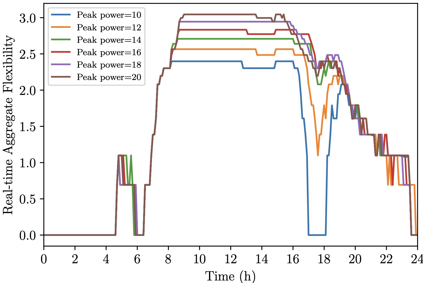
Finally, we demonstrate the effectiveness of this novel flexibility measure using the result in [5]. We consider the problem of measuring real-time flexibility of a workplace EV charging system. The entropy of \(p_t\) at each time is our value-based measure of flexibility. This is intuitive, as higher flexibility indicates more future choices, thus a more uniform distribution and moreover, the objective we try to maximize in the second definition is exactly the logarithm of the size of \(\mathsf{S}\).

This figure shows the change of flexility in a day. We can see from the above figure that the flexibility of the system becomes high during working times as the data we used came from a workplace charging garage. During working hours, EVs arrive and stay in the garage for charging services. The flexibility starts dropping at 5pm when most EVs are leaving. A peak power constraint shrinks the set of feasible actions, thus also reduces the flexility of the system.

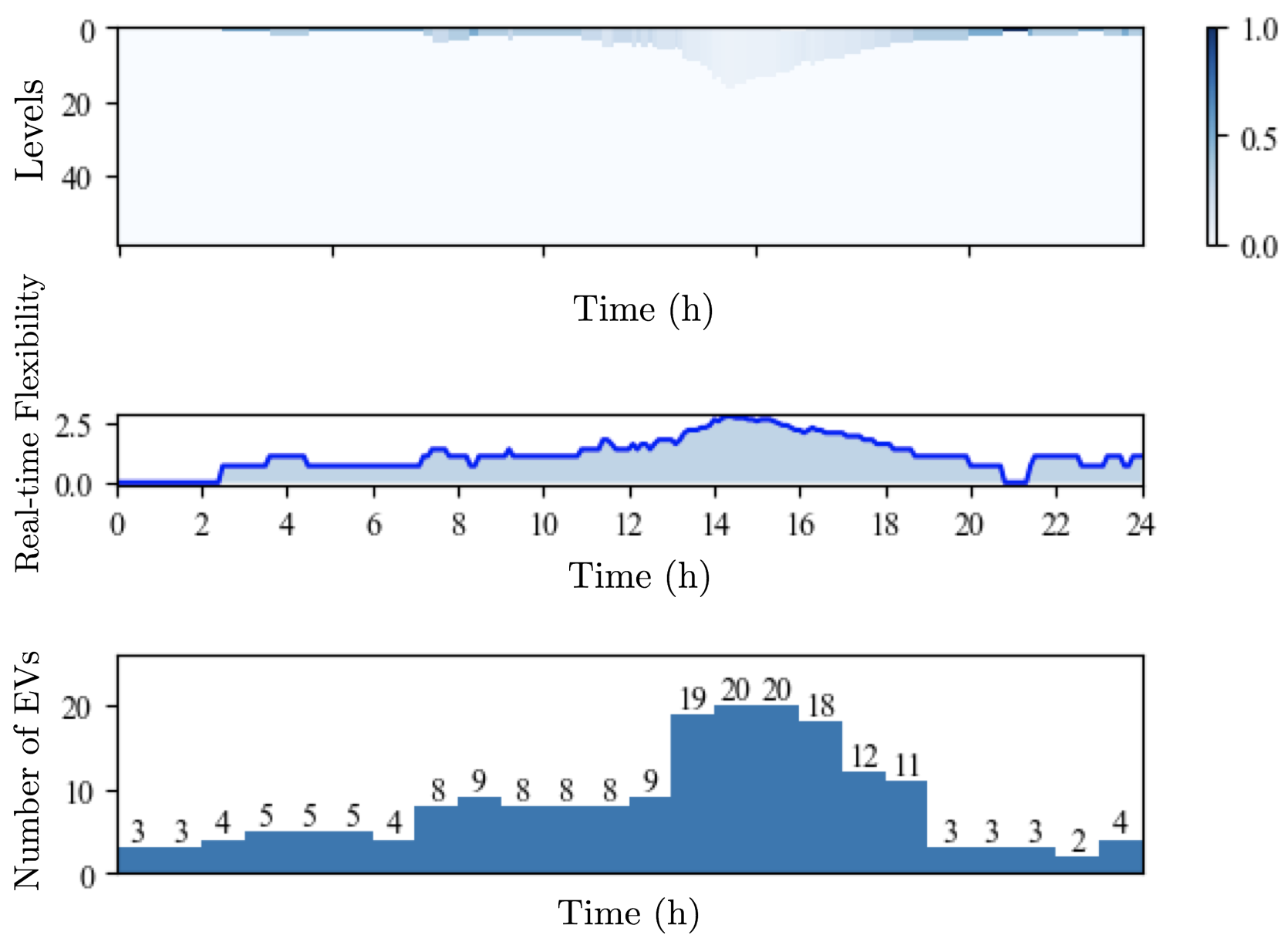
A more detailed daily flexibility dashboard is presented below.

We see the distribution of \(p_t\) in the heatmap atop of the figure and a similar valued-based real-time flexibility curve of a single day in the middle. The bottom figure plots the number of active EVs poltted in an hourly manner. It would be interesting to extend the usage domain of the methods in many other power system applications.

Reference

[1] Li, Tongxin, Bo Sun, Yue Chen, Zixin Ye, Steven H. Low, and Adam Wierman. “Learning-based predictive control via real-time aggregate flexibility.” IEEE Transactions on Smart Grid 12, no. 6 (2021): 4897-4913.

[2] Chen, Xin, Emiliano Dall’Anese, Changhong Zhao, and Na Li. “Aggregate power flexibility in unbalanced distribution systems.” IEEE Transactions on Smart Grid 11, no. 1 (2019): 258-269.

[3] Zhao, Lin, Wei Zhang, He Hao, and Karanjit Kalsi. “A geometric approach to aggregate flexibility modeling of thermostatically controlled loads.” IEEE Transactions on Power Systems 32, no. 6 (2017): 4721-4731.

[4] Werner, Lucien, Adam Wierman, and Steven H. Low. “Pricing flexibility of shiftable demand in electricity markets.” In Proceedings of the Twelfth ACM International Conference on Future Energy Systems, pp. 1-14. 2021.

[5] Li, Tongxin, Steven H. Low, and Adam Wierman. “Real-time flexibility feedback for closed-loop aggregator and system operator coordination.” In Proceedings of the Eleventh ACM International Conference on Future Energy Systems, pp. 279-292. 2020.

[6] Ziebart, Brian D., J. Andrew Bagnell, and Anind K. Dey. “Modeling interaction via the principle of maximum causal entropy.” In ICML. 2010.